Can We Map What We Do Not Know?

THE MISSING LAYER

Maps are very good at showing what has a value and surprisingly poor at showing why a value should be believed. A blue pixel may be a fresh observation. The next blue pixel may be an interpolation between two distant stations. A third may be a model estimate carried forward through a cloudy week. The colour scale treats them as neighbours. Their evidence histories are not.

This volume has accumulated several kinds of absence. The deep ocean may not have been sampled recently. A root-zone value may never have been observed directly. A species may have been missed by a survey. A vessel may have stopped broadcasting. A methane release may have happened between passes. A weather station may never have existed. Calling all of these missing data throws away the most useful information about the gap.

A planetary system therefore needs a second map alongside the map of estimated state: a map of observability. It should describe where evidence exists, when it was collected, what quantity was actually measured, how directly that quantity constrains the displayed variable, and where the system is relying on inference rather than observation.

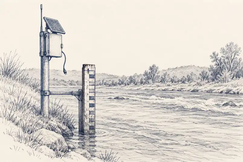
The objective is not to cover the interface in warning labels. It is to make the unknown machine-readable. A system that can represent a river level but cannot represent that the gauge stopped reporting six hours ago has a remarkably specific form of intelligence.

WHAT OBSERVABILITY MEANS

Coverage has more dimensions than a footprint

The simplest coverage map answers one question: where did an instrument collect data? That is useful and incomplete. Observability depends on at least location, time, depth or height, variable, measurement method, detection limit and quality. A float profile and a satellite image may overlap horizontally while observing almost entirely different parts of the ocean.

Freshness is one axis. A groundwater observation from yesterday and one from three years ago may occupy the same coordinate. Directness is another. A radiance measured by an instrument and a root-zone moisture estimate derived through data assimilation should not lose their distinction merely because both end up as numbers. Sampling density matters separately again: one observation inside a 100-kilometre cell is not the same evidential situation as one hundred observations.

Detectability adds a fourth complication. An instrument can have been present and still have had little chance of seeing the phenomenon. Cloud can obstruct optical imagery. A species can occupy a site and escape a survey. A weak plume can fall below a spectrometer's detection threshold. Observation effort and probability of detection belong in the same conversation as the result.

This is why one universal observability score would be tempting and dangerous. A single number would immediately become easier to display and harder to interpret. The useful object is closer to a vector: how recent, how direct, how dense, how detectable, how independently validated and how internally consistent the evidence is for this particular claim.

TYPES OF MISSING EVIDENCE

Zero, unknown, inferred and contradictory need different symbols

A practical observability model begins by refusing to collapse distinct states. Zero means the variable was observed and the measured or estimated quantity was zero. Not observed means there was no usable observation in the relevant window. Below detection means the instrument looked but could not reliably resolve values smaller than a known threshold. These are not formatting variants.

Inferred is different again. Evidence exists, but the displayed state came from a retrieval, interpolation, assimilation system or model rather than a direct measurement of that state. Stale means an observation exists but may no longer represent the present. Unresolved means a signal was detected but could not be assigned a confident identity, as with an environmental DNA sequence that has no close reference.

Contradictory deserves its own state because disagreement is information. Radar may show a vessel where AIS says none exists. A soil probe can disagree with a modelled moisture field. Two satellite retrievals can diverge under difficult atmospheric conditions. Forcing the pipeline to choose one answer too early removes the evidence that something about the system deserves inspection.

These distinctions turn missingness from an empty cell into structured evidence. The system can then ask a useful next question. Is this value absent because the phenomenon is absent, because no sensor looked, because the sensor could not detect it, because the estimate is stale, or because the available observations disagree? Each answer implies a different response.

PROVENANCE AND SENSOR METADATA

Standards already contain much of the machinery

The idea does not require inventing a new language from nothing. The W3C PROV model represents provenance through entities, activities and agents, including how one entity was derived from another and who or what was responsible for producing it. Its purpose is explicitly tied to deciding whether information can be trusted and how it should be combined with other sources.

The Open Geospatial Consortium's SensorThings API handles a more operational layer. An Observation can carry the phenomenon time, the time the result was produced, the observed property, the feature of interest, result quality and the sensor or procedure behind the measurement. In remote sensing, the FeatureOfInterest can be an area or volume rather than a point.

Those fields sound administrative until two datasets disagree. Then the questions become immediate: were they observing the same property, over the same spatial support, at the same time, with comparable methods? Did one result arrive later because it was processed through a retrieval? Which sensor generated it? What quality information travelled with it? Provenance turns a contradiction from two numbers into two traceable claims.

What standards do not automatically provide is the judgement that one region is weakly observed for a particular decision. That has to be computed from metadata, instrument capability and the requirements of the question. The standards supply the grammar. An observability layer would use that grammar to describe the strength and shape of evidence.

AN IGNORANCE LAYER

The map should show where the model is carrying the planet

Imagine a soil-moisture map with a second layer showing time since the last direct satellite constraint, distance to the nearest ground validation site, cloud or radio-frequency interference history, and whether the displayed value is dominated by observation or model propagation. The environmental map would not change. The user's interpretation of it probably would.

The same principle could be applied to an ocean analysis by exposing profile density and age with depth, to biodiversity by showing survey effort and taxonomic reference coverage, to methane by showing usable observation opportunities and detection thresholds, and to shipping by separating broadcast coverage from independent physical detections. Each domain needs different metrics because each domain becomes invisible differently.

For machine systems, the layer could become actionable. A region with high forecast uncertainty and poor recent observation could be prioritised for another satellite acquisition, a float deployment or a field survey. A contradiction between independent sensors could be preserved rather than averaged away. Data collection would then respond not only to where Earth is changing, but to where the system's evidence is weakest.

This is distinct from the uncertainty machinery in Volume 5. Uncertainty describes spread or confidence in an estimate. Observability describes the evidence architecture underneath the estimate. A model can be confidently wrong in a data desert, or uncertain despite dense observations because the physical system is genuinely variable. The two layers should meet without being confused.

WHAT VOLUME 6 ADDS

A blank space is safer than a false sense of coverage

The last century of Earth observation has been a project of filling blanks. Ships sounded the seafloor. Stations measured the atmosphere. Satellites removed continental gaps. Floats entered the ocean. Molecular methods opened hidden biological worlds. Machine learning filled spatial and temporal holes with increasingly capable estimates.

The next problem is not simply to fill the remaining blanks faster. It is to preserve the difference between a blank that was measured, a blank that was inferred, a blank that was never sampled and a blank produced by disagreement. A seamless planetary interface should not require seamless evidence underneath it.

Once those distinctions are represented explicitly, ignorance stops being an embarrassing failure at the edge of the system. It becomes part of the state the system maintains. That allows observation to be allocated where it matters, models to expose where they are extrapolating, and decisions to distinguish absence from absence of evidence.

The planet we still cannot see is therefore not one hidden continent waiting for a future sensor. It is a moving pattern of depths, scales, moments, organisms, institutions and variables that fall outside the current observing geometry. The pattern changes whenever a new instrument is launched or an old station fails. It deserves to be mapped as carefully as everything else.

The most important missing layer may be the one explaining why all the other layers should not be trusted equally.