The Event Happened Between Passes

TEMPORAL OBSERVABILITY

Earth changes continuously. Most observing systems do not observe continuously. A satellite passes at particular times. A field team visits on particular days. A float profiles every ten days. A camera trap wakes when motion triggers it. Between those samples, the system usually assumes that nothing important happened or relies on a model to reconstruct what might have happened.

This creates a blind spot that spatial maps hide particularly well. A location can have excellent nominal coverage and poor temporal observability. If the event lasts two hours and the sensor sees the location every five days, the relevant question is no longer spatial resolution. It is the probability that one of those hours overlaps an observation.

Engineers call the broader problem sampling. A periodic signal sampled too slowly can be misrepresented as a slower pattern or missed entirely. Earth events are usually less cooperative than textbook sine waves: leaks switch on and off, clouds form, animals move, pumps cycle, fires ignite and human activity changes schedules. Irregular events make the sampling problem harder because the frequency to be captured is not known in advance.

SUPER-EMITTERS

Methane made intermittency measurable

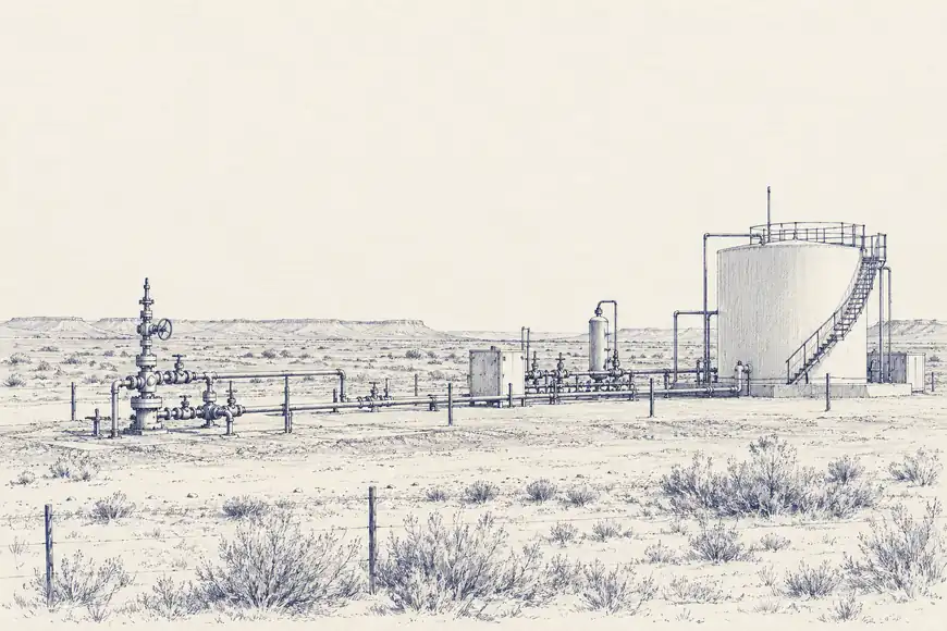
Methane point sources are a clean example because an imaging spectrometer can identify a plume when conditions are suitable and the plume is actually present. NASA and partner airborne surveys over the Permian Basin repeatedly revisited oil and gas infrastructure rather than treating one overflight as a complete inventory.

In a JPL summary of the work, the campaign located 1,756 super-emitting sources across roughly 57,000 square kilometres. Researchers then focused on 1,100 sources observed emitting on at least three flights and classified their persistence from repeated revisits. Only 123 fell into the most persistent class, visible on 50 to 100% of revisits, yet those sources accounted for about 29% of the methane detected from the analysed group.

The important result for observation is not merely that a few sites emitted a lot. It is that presence changed between visits. A facility seen without a plume once cannot be labelled non-emitting in any permanent sense. A facility seen emitting once cannot automatically be assumed to emit continuously. The emission rate and the duty cycle are different variables.

A one-time map collapses them together. Repeat observation separates them. That distinction changes both emissions accounting and mitigation because a persistent malfunction and an intermittent operational release can require different responses. The same sensor becomes more informative simply by returning.

WHEN AN OBSERVATION COUNTS

Revisit time is only the beginning of the clock problem

Satellite specifications often summarize temporal coverage as revisit time, but a geometric revisit is not the same as a usable observation. An optical satellite may pass over a location and find cloud. A thermal instrument may need a particular viewing geometry. A methane spectrometer needs enough reflected sunlight and favourable atmospheric conditions. The calendar contains opportunities, not guarantees.

Constellations improve the odds by distributing observation opportunities across several spacecraft. Geostationary instruments improve them differently by remaining over the same broad region and trading fine spatial detail for high cadence. Ground sensors offer continuous local records while sacrificing global reach. Every architecture buys time with some other constraint.

The useful metric therefore depends on the event. Daily revisit may be excellent for crop development and inadequate for a 30-minute industrial release. A gauge reporting every five minutes may capture a flash rise in one river and say nothing about the neighbouring ungauged catchment. Cadence is meaningful only relative to the duration and speed of the process being observed.

This also explains why more sensors do not automatically remove temporal blind spots. If all of them have similar orbits, cloud dependencies or duty cycles, their gaps can line up. Redundancy helps most when instruments fail differently in time as well as in physics.

THE ABSENCE PROBLEM

Not detected is a statement about a measurement window

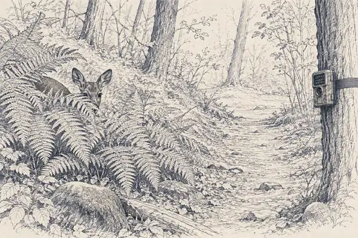
Many Earth datasets turn non-detection into a zero. No plume detected. No vessel detected. No fire detected. No species detected. The zero looks numerical and therefore decisive. In reality, it usually combines at least two possibilities: the event was absent, or the event was present outside the instrument's ability or time window.

Ecology handles this with detection probability and occupancy models: a species can occupy a site while escaping a particular survey. Atmospheric monitoring faces an analogous problem with intermittent emissions. Cloudy remote sensing scenes create it explicitly by carrying masks. The general principle is the same. An observation process has to be modelled separately from the state being observed.

This sounds technical until a dataset is used for compliance. If absence of detection becomes evidence of compliance, temporal sampling becomes part of the legal and financial interpretation. A system designed to find persistent emissions may be poor evidence about short episodic ones even when every individual measurement is accurate.

The cleanest data model therefore distinguishes zero from unknown and unknown from not observed. These are three different states. Databases frequently compress them because one column is convenient. Earth continues to exploit the distinction.

MATCHING CADENCE TO PROCESS

Every phenomenon has its own observation clock

The answer is not continuous observation of everything. That would move the problem from sensing to bandwidth, storage, energy, calibration and attention. The useful architecture matches observation cadence to how quickly a variable can change and how costly it is to miss the change.

Slow variables can tolerate sparse sampling if their dynamics are well constrained. Fast variables need higher cadence or event-triggered observation. Processes with uncertain timing benefit from heterogeneous networks so that one instrument can catch what another misses. Models can bridge intervals, but the system should keep track of how long it has been since reality last corrected the estimate.

Volume 5 described systems that can retask sensors when uncertainty rises. The point here is earlier in the chain: without a model of temporal observability, the system may not know that uncertainty should have risen at all. A blank interval can look deceptively calm.

The event did not become invisible. It simply happened while the observing system was elsewhere.